R and SQL (Part 2)
This is part 2 of a series of posts demonstrating how equivalent analysis can be carried out in SQL and R. Here we look at joins, grouped data, and subqueries.
Introduction
In Part 1 of this series we looked at the similarities between SQL and R when selecting, sorting and filtering data. In this second part we are going to extend the comparison to include joins, grouped data and subqueries.
The data
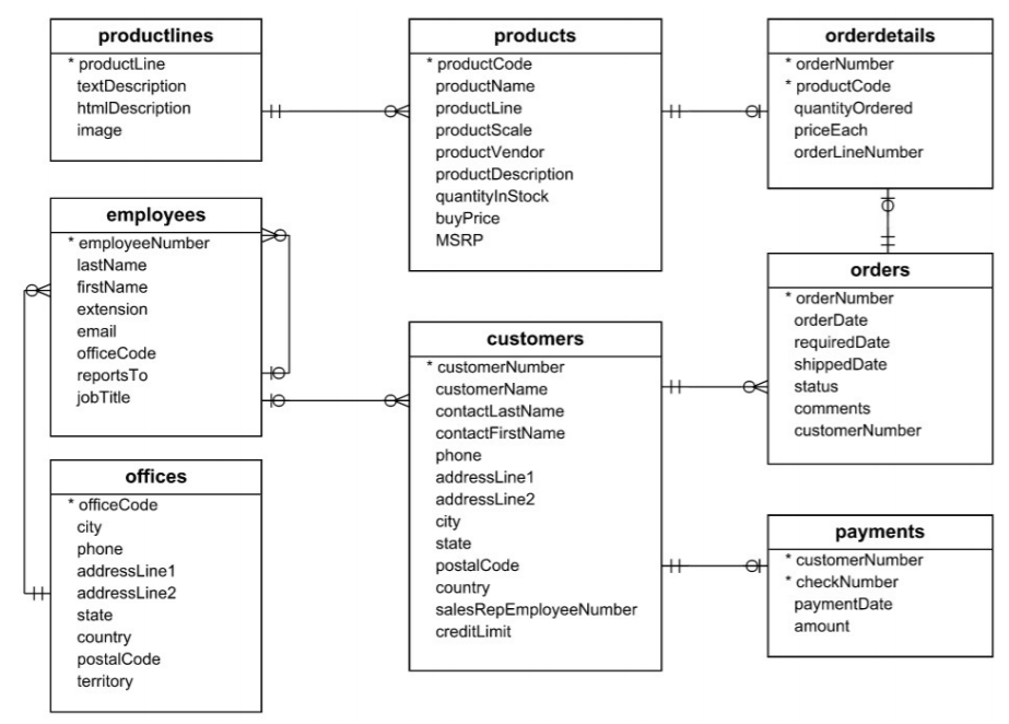
We will use the same sample dataset from mysqltutorial.org that was used in the first part of this post, as described here. The schema is reproduced below for ease of reference:
Instructions on how to load the sample dataset into MySQL and R were provided here.
1. Common joins
A join allows you to combine variables or columns from two tables. It first matches observations by their keys, then copies across variables from one table to another.
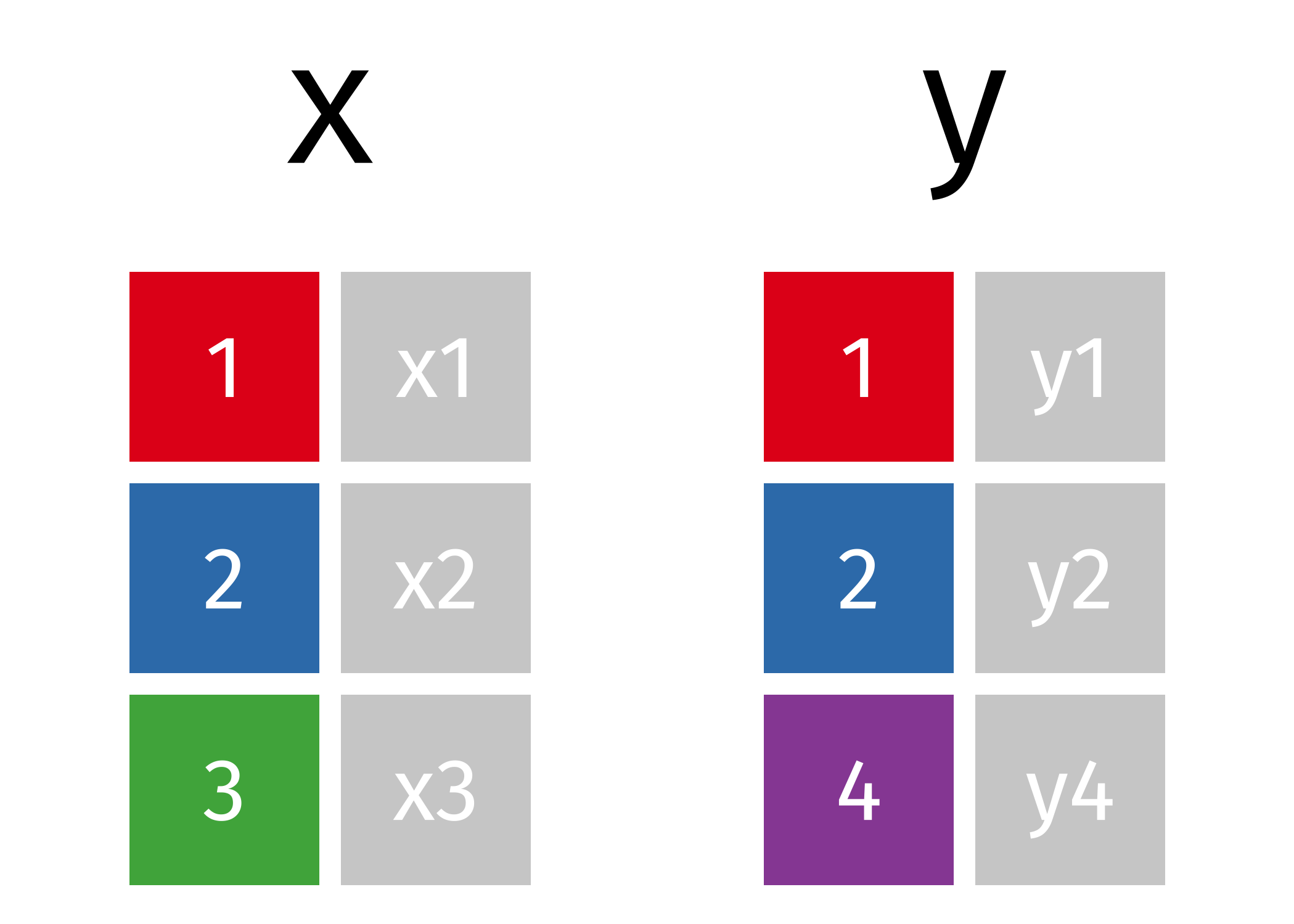
To understand joins, we are going to use the explanation provided by Hadley Wickham in R for Data Science, and the excellent animations that were produced by Garrick Aden-Buie. These illustrate the different ways that we can join the data in table x, below, with the data in table y. The colored columns represent the “key” variable that is used to match the rows between the tables.
This section looks at four common joins:
- Inner join
- Left join
- Right join
- Full join
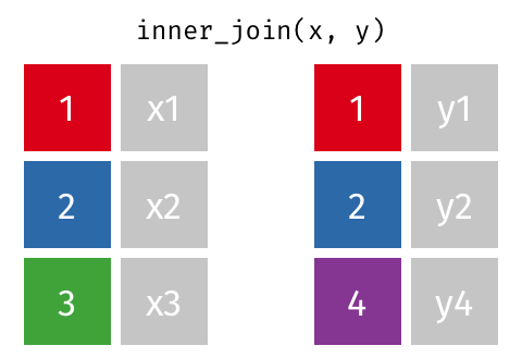
1.1 Inner join
An inner join shows all rows from x where there are matching values in y, and all columns from x and y:
Example 1.1a:
Say we want to list the name of every employee from the employees table who has one or more customers recorded in the customers table.
This is an example of an inner join, as we only want records that have a match in both tables. In this case our keys - the columns that we will be matching - are the employeeNumber in the employees table and the salesRepEmployeeNumber in the customers table.
We would like the code to return the following information:
- employee number
- employee first name
- employee second name
- customer name(s)
With SQL:
To do this in SQL we would use INNER JOIN, followed by the name of the table we are joining to. We then use ON to specify the names of the columns (keys) that are being used to match the data in the two tables:
SELECT
  employees.employeeNumber,
  employees.lastName,
  employees.firstName,
  customers.customerName
FROM
  employees
  INNER JOIN
  customers
    ON employees.employeeNumber = customers.salesRepEmployeeNumber
ORDER BY
  lastName, customerName
Note that we’ve specified the table from which each column is taken; for example, using employees.employeeNumber rather than just employeeNumber. This is necessary in cases where the same column name appears in more than one table. In this particular example, we could have written the code without the table prefixes, but they have been included for illustrative purposes.
With R:
The same join could be carried out in R using the inner_join function. This includes the by argument (equivalent to SQL’s ON), in which we list the names of the keys:
employees %>%   #left-hand table
  #after 'by' we list the key from the left-hand table first:
  inner_join(customers, by = c("employeeNumber" = "salesRepEmployeeNumber")) %>%
  select(employeeNumber, lastName, firstName, customerName) %>%
arrange(lastName, customerName)| employeeNumber | lastName | firstName | customerName |
|---|---|---|---|
| 1337 | Bondur | Loui | Auto Canal+ Petit |
| 1337 | Bondur | Loui | La Corne D’abondance, Co. |
| 1337 | Bondur | Loui | Lyon Souveniers |
| 1337 | Bondur | Loui | Marseille Mini Autos |
| 1337 | Bondur | Loui | Reims Collectables |
| 1337 | Bondur | Loui | Saveley & Henriot, Co. |
| 1501 | Bott | Larry | AV Stores, Co. |
| 1501 | Bott | Larry | Double Decker Gift Stores, Ltd |
| 1501 | Bott | Larry | giftsbymail.co.uk |
| 1501 | Bott | Larry | Oulu Toy Supplies, Inc. |
| 1501 | Bott | Larry | Stylish Desk Decors, Co. |
| 1501 | Bott | Larry | Suominen Souveniers |
| 1501 | Bott | Larry | Toys of Finland, Co. |
| 1501 | Bott | Larry | UK Collectables, Ltd. |
| 1401 | Castillo | Pamela | Amica Models & Co. |
| 1401 | Castillo | Pamela | Danish Wholesale Imports |
| 1401 | Castillo | Pamela | Frau da Collezione |
| 1401 | Castillo | Pamela | Heintze Collectables |
| 1401 | Castillo | Pamela | L’ordine Souveniers |
| 1401 | Castillo | Pamela | Mini Auto Werke |
| 1401 | Castillo | Pamela | Petit Auto |
| 1401 | Castillo | Pamela | Rovelli Gifts |
| 1401 | Castillo | Pamela | Royale Belge |
| 1401 | Castillo | Pamela | Salzburg Collectables |
| 1188 | Firrelli | Julie | Cambridge Collectables Co. |
| 1188 | Firrelli | Julie | Classic Gift Ideas, Inc |
| 1188 | Firrelli | Julie | Collectables For Less Inc. |
| 1188 | Firrelli | Julie | Diecast Collectables |
| 1188 | Firrelli | Julie | Mini Creations Ltd. |
| 1188 | Firrelli | Julie | Online Mini Collectables |
| 1611 | Fixter | Andy | Anna’s Decorations, Ltd |
| 1611 | Fixter | Andy | Australian Collectables, Ltd |
| 1611 | Fixter | Andy | Australian Collectors, Co. |
| 1611 | Fixter | Andy | Australian Gift Network, Co |
| 1611 | Fixter | Andy | Souveniers And Things Co. |
| 1702 | Gerard | Martin | CAF Imports |
| 1702 | Gerard | Martin | Corrida Auto Replicas, Ltd |
| 1702 | Gerard | Martin | Enaco Distributors |
| 1702 | Gerard | Martin | Iberia Gift Imports, Corp. |
| 1702 | Gerard | Martin | Precious Collectables |
| 1702 | Gerard | Martin | Vida Sport, Ltd |
| 1370 | Hernandez | Gerard | Alpha Cognac |
| 1370 | Hernandez | Gerard | Atelier graphique |
| 1370 | Hernandez | Gerard | Auto Associés & Cie. |
| 1370 | Hernandez | Gerard | Daedalus Designs Imports |
| 1370 | Hernandez | Gerard | Euro+ Shopping Channel |
| 1370 | Hernandez | Gerard | La Rochelle Gifts |
| 1370 | Hernandez | Gerard | Mini Caravy |
| 1165 | Jennings | Leslie | Corporate Gift Ideas Co. |
| 1165 | Jennings | Leslie | Mini Gifts Distributors Ltd. |
| 1165 | Jennings | Leslie | Mini Wheels Co. |
| 1165 | Jennings | Leslie | Signal Collectibles Ltd. |
| 1165 | Jennings | Leslie | Technics Stores Inc. |
| 1165 | Jennings | Leslie | The Sharp Gifts Warehouse |
| 1504 | Jones | Barry | Baane Mini Imports |
| 1504 | Jones | Barry | Bavarian Collectables Imports, Co. |
| 1504 | Jones | Barry | Blauer See Auto, Co. |
| 1504 | Jones | Barry | Clover Collections, Co. |
| 1504 | Jones | Barry | Herkku Gifts |
| 1504 | Jones | Barry | Norway Gifts By Mail, Co. |
| 1504 | Jones | Barry | Scandinavian Gift Ideas |
| 1504 | Jones | Barry | Toms Spezialitäten, Ltd |
| 1504 | Jones | Barry | Volvo Model Replicas, Co |
| 1612 | Marsh | Peter | Down Under Souveniers, Inc |
| 1612 | Marsh | Peter | Extreme Desk Decorations, Ltd |
| 1612 | Marsh | Peter | GiftsForHim.com |
| 1612 | Marsh | Peter | Handji Gifts& Co |
| 1612 | Marsh | Peter | Kelly’s Gift Shop |
| 1621 | Nishi | Mami | Cruz & Sons Co. |
| 1621 | Nishi | Mami | Dragon Souveniers, Ltd. |
| 1621 | Nishi | Mami | King Kong Collectables, Co. |
| 1621 | Nishi | Mami | Osaka Souveniers Co. |
| 1621 | Nishi | Mami | Tokyo Collectables, Ltd |
| 1216 | Patterson | Steve | Auto-Moto Classics Inc. |
| 1216 | Patterson | Steve | Diecast Classics Inc. |
| 1216 | Patterson | Steve | FunGiftIdeas.com |
| 1216 | Patterson | Steve | Gifts4AllAges.com |
| 1216 | Patterson | Steve | Marta’s Replicas Co. |
| 1216 | Patterson | Steve | Online Diecast Creations Co. |
| 1166 | Thompson | Leslie | Boards & Toys Co. |
| 1166 | Thompson | Leslie | Collectable Mini Designs Co. |
| 1166 | Thompson | Leslie | Men ‘R’ US Retailers, Ltd. |
| 1166 | Thompson | Leslie | Signal Gift Stores |
| 1166 | Thompson | Leslie | Toys4GrownUps.com |
| 1166 | Thompson | Leslie | West Coast Collectables Co. |
| 1286 | Tseng | Foon Yue | American Souvenirs Inc |
| 1286 | Tseng | Foon Yue | Classic Legends Inc. |
| 1286 | Tseng | Foon Yue | Microscale Inc. |
| 1286 | Tseng | Foon Yue | Muscle Machine Inc |
| 1286 | Tseng | Foon Yue | Québec Home Shopping Network |
| 1286 | Tseng | Foon Yue | Super Scale Inc. |
| 1286 | Tseng | Foon Yue | Vitachrome Inc. |
| 1323 | Vanauf | George | Canadian Gift Exchange Network |
| 1323 | Vanauf | George | Gift Depot Inc. |
| 1323 | Vanauf | George | Gift Ideas Corp. |
| 1323 | Vanauf | George | Land of Toys Inc. |
| 1323 | Vanauf | George | Mini Classics |
| 1323 | Vanauf | George | Motor Mint Distributors Inc. |
| 1323 | Vanauf | George | Royal Canadian Collectables, Ltd. |
| 1323 | Vanauf | George | Tekni Collectables Inc. |
Example 1.1b:
Say that we wanted to list every customer from the customers table who has one or more orders in the orders table.
This is another example of an inner join, this time matching records using the ‘customerNumber’ column as our key, which is the same in both tables.
We want the query to return the following information:
- customer number
- customer name
- order number
- current order status
With SQL:
The fact that the same column name is used in both tables means we can simplify our code with USING instead of ON, as follows:
SELECT
  c.customerNumber,
  c.customerName,
  o.orderNumber,
  o.status
FROM
  customers AS c
  INNER JOIN
  orders AS o
    USING (customerNumber)
ORDER BY
  customerName
This simplifies the code as we only need to list one column after USING.
In the example above, we’ve also used aliases in place of the full table names, which further simplifies the code. This has assigned the short name ‘c’ to the ‘customers’ table and ‘o’ to the ‘orders’ table. This is done with the keyword AS, though even this could be excluded. Aliases makes the code shorter and easier to read.
With R:
The equivalent R code is shown below. Note that we now only need to specify the one column name in the by argument.
customers %>%
  inner_join(orders, by = "customerNumber") %>%
  select(customerNumber, customerName, orderNumber, status) %>%
arrange(customerName)| customerNumber | customerName | orderNumber | status |
|---|---|---|---|
| 242 | Alpha Cognac | 10136 | Shipped |
| 242 | Alpha Cognac | 10178 | Shipped |
| 242 | Alpha Cognac | 10397 | Shipped |
| 249 | Amica Models & Co. | 10280 | Shipped |
| 249 | Amica Models & Co. | 10293 | Shipped |
| 276 | Anna’s Decorations, Ltd | 10148 | Shipped |
| 276 | Anna’s Decorations, Ltd | 10169 | Shipped |
| 276 | Anna’s Decorations, Ltd | 10370 | Shipped |
| 276 | Anna’s Decorations, Ltd | 10391 | Shipped |
| 103 | Atelier graphique | 10123 | Shipped |
| 103 | Atelier graphique | 10298 | Shipped |
| 103 | Atelier graphique | 10345 | Shipped |
| 471 | Australian Collectables, Ltd | 10193 | Shipped |
| 471 | Australian Collectables, Ltd | 10265 | Shipped |
| 471 | Australian Collectables, Ltd | 10415 | Disputed |
| 114 | Australian Collectors, Co. | 10120 | Shipped |
| 114 | Australian Collectors, Co. | 10125 | Shipped |
| 114 | Australian Collectors, Co. | 10223 | Shipped |
| 114 | Australian Collectors, Co. | 10342 | Shipped |
| 114 | Australian Collectors, Co. | 10347 | Shipped |
| 333 | Australian Gift Network, Co | 10152 | Shipped |
| 333 | Australian Gift Network, Co | 10174 | Shipped |
| 333 | Australian Gift Network, Co | 10374 | Shipped |
| 198 | Auto-Moto Classics Inc. | 10130 | Shipped |
| 198 | Auto-Moto Classics Inc. | 10290 | Shipped |
| 198 | Auto-Moto Classics Inc. | 10352 | Shipped |
| 256 | Auto Associés & Cie. | 10216 | Shipped |
| 256 | Auto Associés & Cie. | 10304 | Shipped |
| 406 | Auto Canal+ Petit | 10211 | Shipped |
| 406 | Auto Canal+ Petit | 10252 | Shipped |
| 406 | Auto Canal+ Petit | 10402 | Shipped |
| 187 | AV Stores, Co. | 10110 | Shipped |
| 187 | AV Stores, Co. | 10306 | Shipped |
| 187 | AV Stores, Co. | 10332 | Shipped |
| 121 | Baane Mini Imports | 10103 | Shipped |
| 121 | Baane Mini Imports | 10158 | Shipped |
| 121 | Baane Mini Imports | 10309 | Shipped |
| 121 | Baane Mini Imports | 10325 | Shipped |
| 415 | Bavarian Collectables Imports, Co. | 10296 | Shipped |
| 128 | Blauer See Auto, Co. | 10101 | Shipped |
| 128 | Blauer See Auto, Co. | 10230 | Shipped |
| 128 | Blauer See Auto, Co. | 10300 | Shipped |
| 128 | Blauer See Auto, Co. | 10323 | Shipped |
| 219 | Boards & Toys Co. | 10154 | Shipped |
| 219 | Boards & Toys Co. | 10376 | Shipped |
| 344 | CAF Imports | 10177 | Shipped |
| 344 | CAF Imports | 10231 | Shipped |
| 173 | Cambridge Collectables Co. | 10228 | Shipped |
| 173 | Cambridge Collectables Co. | 10249 | Shipped |
| 202 | Canadian Gift Exchange Network | 10206 | Shipped |
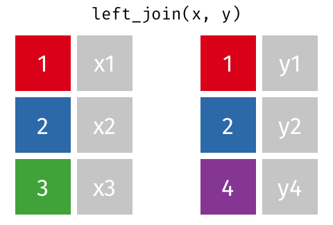
1.2 Left join
A left join (or outer left join) returns all rows from x, and all columns from x and y. Rows in x with no match in y will have NA or NULL values in the new columns.
Example 1.2:
In the example above we wanted to see the names customers in the customers table who had a corresponding order in the orders table. But what if we wanted to see names of all customers and their order information, even if they don’t have any orders?
This is an example of a left join. We can do this using LEFT JOIN in SQL and left_join in R, as follows:
With SQL:
SELECT
  c.customerNumber,
  c.customerName,
  o.orderNumber,
  o.status
FROM
  customers AS c
  LEFT JOIN
  orders AS o
    ON c.customerNumber = o.customerNumber
ORDER BY customerName
With R:
customers %>%
  left_join(orders, by = "customerNumber") %>%
  select(customerNumber, customerName, orderNumber, status) %>%
  arrange(customerName)
This returns 350 records, the first 50 of which are shown in the table below. If you scroll down, you will see that some customers have ‘NA’ for orderNumber and status (this will appear as ‘NULL’ in MySQL). These are customers who had no corresponding orders in the orders table. Note that each customer will appear more than once if they have more than one order.
| customerNumber | customerName | orderNumber | status |
|---|---|---|---|
| 242 | Alpha Cognac | 10136 | Shipped |
| 242 | Alpha Cognac | 10178 | Shipped |
| 242 | Alpha Cognac | 10397 | Shipped |
| 168 | American Souvenirs Inc | NA | NA |
| 249 | Amica Models & Co. | 10280 | Shipped |
| 249 | Amica Models & Co. | 10293 | Shipped |
| 237 | ANG Resellers | NA | NA |
| 276 | Anna’s Decorations, Ltd | 10148 | Shipped |
| 276 | Anna’s Decorations, Ltd | 10169 | Shipped |
| 276 | Anna’s Decorations, Ltd | 10370 | Shipped |
| 276 | Anna’s Decorations, Ltd | 10391 | Shipped |
| 465 | Anton Designs, Ltd. | NA | NA |
| 206 | Asian Shopping Network, Co | NA | NA |
| 348 | Asian Treasures, Inc. | NA | NA |
| 103 | Atelier graphique | 10123 | Shipped |
| 103 | Atelier graphique | 10298 | Shipped |
| 103 | Atelier graphique | 10345 | Shipped |
| 471 | Australian Collectables, Ltd | 10193 | Shipped |
| 471 | Australian Collectables, Ltd | 10265 | Shipped |
| 471 | Australian Collectables, Ltd | 10415 | Disputed |
| 114 | Australian Collectors, Co. | 10120 | Shipped |
| 114 | Australian Collectors, Co. | 10125 | Shipped |
| 114 | Australian Collectors, Co. | 10223 | Shipped |
| 114 | Australian Collectors, Co. | 10342 | Shipped |
| 114 | Australian Collectors, Co. | 10347 | Shipped |
| 333 | Australian Gift Network, Co | 10152 | Shipped |
| 333 | Australian Gift Network, Co | 10174 | Shipped |
| 333 | Australian Gift Network, Co | 10374 | Shipped |
| 198 | Auto-Moto Classics Inc. | 10130 | Shipped |
| 198 | Auto-Moto Classics Inc. | 10290 | Shipped |
| 198 | Auto-Moto Classics Inc. | 10352 | Shipped |
| 256 | Auto Associés & Cie. | 10216 | Shipped |
| 256 | Auto Associés & Cie. | 10304 | Shipped |
| 406 | Auto Canal+ Petit | 10211 | Shipped |
| 406 | Auto Canal+ Petit | 10252 | Shipped |
| 406 | Auto Canal+ Petit | 10402 | Shipped |
| 187 | AV Stores, Co. | 10110 | Shipped |
| 187 | AV Stores, Co. | 10306 | Shipped |
| 187 | AV Stores, Co. | 10332 | Shipped |
| 121 | Baane Mini Imports | 10103 | Shipped |
| 121 | Baane Mini Imports | 10158 | Shipped |
| 121 | Baane Mini Imports | 10309 | Shipped |
| 121 | Baane Mini Imports | 10325 | Shipped |
| 415 | Bavarian Collectables Imports, Co. | 10296 | Shipped |
| 293 | BG&E Collectables | NA | NA |
| 128 | Blauer See Auto, Co. | 10101 | Shipped |
| 128 | Blauer See Auto, Co. | 10230 | Shipped |
| 128 | Blauer See Auto, Co. | 10300 | Shipped |
| 128 | Blauer See Auto, Co. | 10323 | Shipped |
| 219 | Boards & Toys Co. | 10154 | Shipped |
1.3 Right join
A right join (or outer right join) returns all rows from y, and all columns from x and y. Rows in y with no match in x will have NA or NULL values in the new columns.
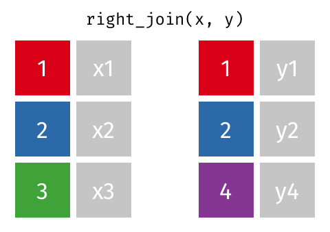
This is exactly the same as a left join, described in the section above, but this time we’re returning all rows from the right-hand table (in this case, y) rather than those from the left-hand table.
A right join in which y is designated as the right-hand table (as in the animation above) would give exactly the same result as a left join in which y was designated as the left-hand table. The choice of whether a table is designated on the left or the right is entirely arbitrary.
Right joins can be carried out using RIGHT JOIN in SQL and right_join in R. No example is provided here given the similarity to left joins.
1.4 Full join
A full join (or full outer join) returns all rows and all columns from both x and y. Where there is no match for a particular key value, the missing values will appear as NA or NULL.
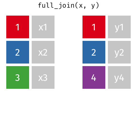
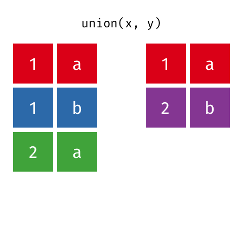
Full joins are not actually supported in MySQL. However, a full join is equivalent to a combination of a left join and right join, as described above. To combine the results of these two joins, we need to use union.
Union returns all unique rows from tables x and y as follows:
Example 1.4:
Say we want to list the name of every employee from the employees table, and every customer from the customers table. Where possible, we want to match the name of each employee to his/her customers. However we also want to return the names of all employees without customers, and the names of all customers without an associated employee. This is an example of a full join.
Assume that we want our query to return:
- each employee’s last name
- each employee’s first name
- each customer’s name
With SQL:
To simulate a full join in SQL, we are going to use a LEFT JOIN, a RIGHT JOIN and the UNION of the two, as follows:
SELECT
  e.lastName, e.firstName, c.customerName
FROM
  employees AS e
  LEFT JOIN
  customers AS c
    ON e.employeeNumber = c.salesRepEmployeeNumber

UNION

SELECT
  e.lastName, e.firstName, c.customerName
FROM
  employees AS e
  RIGHT JOIN
  customers AS c
    ON e.employeeNumber = c.salesRepEmployeeNumber
With R:
In R, the syntax is much simpler as we can use full_join:
employees %>%
  full_join(customers, by = c('employeeNumber' = 'salesRepEmployeeNumber')) %>%
  select(lastName, firstName, customerName)
The two sets of code above return the following 130 records. As expected, this shows the name of each employee matched to their customer(s), where such a match exists, but also the names of each employee and customer even if there is no match:
| lastName | firstName | customerName |
|---|---|---|
| Murphy | Diane | NA |
| Patterson | Mary | NA |
| Firrelli | Jeff | NA |
| Patterson | William | NA |
| Bondur | Gerard | NA |
| Bow | Anthony | NA |
| Jennings | Leslie | Mini Gifts Distributors Ltd. |
| Jennings | Leslie | Mini Wheels Co. |
| Jennings | Leslie | Technics Stores Inc. |
| Jennings | Leslie | Corporate Gift Ideas Co. |
| Jennings | Leslie | The Sharp Gifts Warehouse |
| Jennings | Leslie | Signal Collectibles Ltd. |
| Thompson | Leslie | Signal Gift Stores |
| Thompson | Leslie | Toys4GrownUps.com |
| Thompson | Leslie | Boards & Toys Co. |
| Thompson | Leslie | Collectable Mini Designs Co. |
| Thompson | Leslie | Men ‘R’ US Retailers, Ltd. |
| Thompson | Leslie | West Coast Collectables Co. |
| Firrelli | Julie | Cambridge Collectables Co. |
| Firrelli | Julie | Online Mini Collectables |
| Firrelli | Julie | Mini Creations Ltd. |
| Firrelli | Julie | Classic Gift Ideas, Inc |
| Firrelli | Julie | Collectables For Less Inc. |
| Firrelli | Julie | Diecast Collectables |
| Patterson | Steve | Diecast Classics Inc. |
| Patterson | Steve | Auto-Moto Classics Inc. |
| Patterson | Steve | Marta’s Replicas Co. |
| Patterson | Steve | Gifts4AllAges.com |
| Patterson | Steve | Online Diecast Creations Co. |
| Patterson | Steve | FunGiftIdeas.com |
| Tseng | Foon Yue | Muscle Machine Inc |
| Tseng | Foon Yue | American Souvenirs Inc |
| Tseng | Foon Yue | Vitachrome Inc. |
| Tseng | Foon Yue | Québec Home Shopping Network |
| Tseng | Foon Yue | Classic Legends Inc. |
| Tseng | Foon Yue | Super Scale Inc. |
| Tseng | Foon Yue | Microscale Inc. |
| Vanauf | George | Land of Toys Inc. |
| Vanauf | George | Gift Depot Inc. |
| Vanauf | George | Canadian Gift Exchange Network |
| Vanauf | George | Royal Canadian Collectables, Ltd. |
| Vanauf | George | Mini Classics |
| Vanauf | George | Tekni Collectables Inc. |
| Vanauf | George | Gift Ideas Corp. |
| Vanauf | George | Motor Mint Distributors Inc. |
| Bondur | Loui | Saveley & Henriot, Co. |
| Bondur | Loui | La Corne D’abondance, Co. |
| Bondur | Loui | Lyon Souveniers |
| Bondur | Loui | Marseille Mini Autos |
| Bondur | Loui | Reims Collectables |
| Bondur | Loui | Auto Canal+ Petit |
| Hernandez | Gerard | Atelier graphique |
| Hernandez | Gerard | La Rochelle Gifts |
| Hernandez | Gerard | Euro+ Shopping Channel |
| Hernandez | Gerard | Daedalus Designs Imports |
| Hernandez | Gerard | Mini Caravy |
| Hernandez | Gerard | Alpha Cognac |
| Hernandez | Gerard | Auto Associés & Cie. |
| Castillo | Pamela | Danish Wholesale Imports |
| Castillo | Pamela | Heintze Collectables |
| Castillo | Pamela | Amica Models & Co. |
| Castillo | Pamela | Rovelli Gifts |
| Castillo | Pamela | Petit Auto |
| Castillo | Pamela | Royale Belge |
| Castillo | Pamela | Salzburg Collectables |
| Castillo | Pamela | L’ordine Souveniers |
| Castillo | Pamela | Mini Auto Werke |
| Castillo | Pamela | Frau da Collezione |
| Bott | Larry | Toys of Finland, Co. |
| Bott | Larry | AV Stores, Co. |
| Bott | Larry | UK Collectables, Ltd. |
| Bott | Larry | giftsbymail.co.uk |
| Bott | Larry | Oulu Toy Supplies, Inc. |
| Bott | Larry | Stylish Desk Decors, Co. |
| Bott | Larry | Suominen Souveniers |
| Bott | Larry | Double Decker Gift Stores, Ltd |
| Jones | Barry | Baane Mini Imports |
| Jones | Barry | Blauer See Auto, Co. |
| Jones | Barry | Volvo Model Replicas, Co |
| Jones | Barry | Herkku Gifts |
| Jones | Barry | Clover Collections, Co. |
| Jones | Barry | Toms Spezialitäten, Ltd |
| Jones | Barry | Norway Gifts By Mail, Co. |
| Jones | Barry | Bavarian Collectables Imports, Co. |
| Jones | Barry | Scandinavian Gift Ideas |
| Fixter | Andy | Australian Collectors, Co. |
| Fixter | Andy | Anna’s Decorations, Ltd |
| Fixter | Andy | Souveniers And Things Co. |
| Fixter | Andy | Australian Gift Network, Co |
| Fixter | Andy | Australian Collectables, Ltd |
| Marsh | Peter | Handji Gifts& Co |
| Marsh | Peter | Down Under Souveniers, Inc |
| Marsh | Peter | GiftsForHim.com |
| Marsh | Peter | Extreme Desk Decorations, Ltd |
| Marsh | Peter | Kelly’s Gift Shop |
| King | Tom | NA |
| Nishi | Mami | Dragon Souveniers, Ltd. |
| Nishi | Mami | Osaka Souveniers Co. |
| Nishi | Mami | King Kong Collectables, Co. |
| Nishi | Mami | Cruz & Sons Co. |
| Nishi | Mami | Tokyo Collectables, Ltd |
| Kato | Yoshimi | NA |
| Gerard | Martin | Enaco Distributors |
| Gerard | Martin | Vida Sport, Ltd |
| Gerard | Martin | CAF Imports |
| Gerard | Martin | Precious Collectables |
| Gerard | Martin | Corrida Auto Replicas, Ltd |
| Gerard | Martin | Iberia Gift Imports, Corp. |
| NA | NA | Havel & Zbyszek Co |
| NA | NA | Porto Imports Co. |
| NA | NA | Asian Shopping Network, Co |
| NA | NA | Natürlich Autos |
| NA | NA | ANG Resellers |
| NA | NA | Messner Shopping Network |
| NA | NA | Franken Gifts, Co |
| NA | NA | BG&E Collectables |
| NA | NA | Schuyler Imports |
| NA | NA | Der Hund Imports |
| NA | NA | Cramer Spezialitäten, Ltd |
| NA | NA | Asian Treasures, Inc. |
| NA | NA | SAR Distributors, Co |
| NA | NA | Kommission Auto |
| NA | NA | Lisboa Souveniers, Inc |
| NA | NA | Stuttgart Collectable Exchange |
| NA | NA | Feuer Online Stores, Inc |
| NA | NA | Warburg Exchange |
| NA | NA | Anton Designs, Ltd. |
| NA | NA | Mit Vergnügen & Co. |
| NA | NA | Kremlin Collectables, Co. |
| NA | NA | Raanan Stores, Inc |
2. Grouped data
In SQL and R, it is possible to group a set of rows into a summary row. This summary row can include an aggregate measure of each group; for example, the sum, the average, or the count of records in each group.
It is also possible to filter the data based on these aggregates. For example, you could filter to only show rows from groups with more than 20 records, or only show rows from groups where the average value of a certain variable was greater than 100.
2.1 Summarizing grouped data
Grouped data is often summarized using aggregate functions such as SUM, AVG, MAX, MIN and COUNT. Here we look at a couple of examples using our sample database.
Example A
Say we want to find the total value (in $) of each order in our sample data set.
To do this, we need to (1) calculate the value of each product in every order, i.e. the quantity times the price; and (2) group each product sold by its order number and add these values together.
With SQL:
In SQL we group the data using the GROUP BY clause, and specify our aggregate calculation in the SELECT clause, as follows:
SELECT
  orderNumber,
  SUM(quantityOrdered * priceEach) AS value
FROM
  orderdetails
GROUP BY
  orderNumber
With R:
In R, we would use group_by() to group the data, and summarize() to apply the aggregate function to each group:
orderdetails %>%
  group_by(orderNumber) %>%
  summarize(value = sum(quantityOrdered * priceEach)) %>%
  select(orderNumber, value)
The first 10 records (out of 326) are shown in the table below:
## `summarise()` ungrouping output (override with `.groups` argument)| orderNumber | value |
|---|---|
| 10100 | 10223.83 |
| 10101 | 10549.01 |
| 10102 | 5494.78 |
| 10103 | 50218.95 |
| 10104 | 40206.20 |
| 10105 | 53959.21 |
| 10106 | 52151.81 |
| 10107 | 22292.62 |
| 10108 | 51001.22 |
| 10109 | 25833.14 |
Example B
We can also group using an expression rather than values that already exist in a column.
For example, say we wanted to find the total value of orders in each year, where the order has been shipped.
To do this, we need to do a combination of the following:
- Join the orders table, which has the date of each order, with the orderdetails table, which contains information on the quantity and price of the products ordered
- Use the
YEAR()function in SQL, andyear()in R (using the lubridate package), which the returns the year corresponding to each order date. This is will be used to group the data - Filter the data to only include orders whose status is ‘shipped’.
This can be done in the following code:
With SQL:
SELECT
  YEAR(orderDate) AS year,
  SUM(quantityOrdered * priceEach) AS value
FROM
  orders
  INNER JOIN
  orderdetails
    USING (orderNumber)
WHERE
  status = 'Shipped'
GROUP BY
  YEAR(orderDate)
With R:
orders %>%
  inner_join(orderdetails, by = 'orderNumber') %>%
  filter(status == 'Shipped') %>%
  group_by(year = lubridate::year(orderDate)) %>%
  summarize(value = sum(quantityOrdered * priceEach))
Which gives the total value of shipped orders for the three years:
## `summarise()` ungrouping output (override with `.groups` argument)| year | value |
|---|---|
| 2003 | 3223096 |
| 2004 | 4300603 |
| 2005 | 1341396 |
2.2 Filtering grouped data
In SQL and R we can specify filter conditions for a group of rows. This assumes that we have already grouped our data using GROUP BY in SQL or group_by() in R.
When filtering grouped data in SQL we use the HAVING clause. Note that we do not use the WHERE clause, which is only used to filter ungrouped data.
In R, we filter our grouped data using filter(), which was also used with ungrouped data.
Example A
Say we want to show all order numbers in which more than 650 individual items were ordered. This requires us to group by order number (orderNumber) from the orderdetails table, and to filter the results based on the total quantity of products in each order.
With SQL:
In SQL we apply our filter using the HAVING clause, as follows:
SELECT
  orderNumber,
  sum(quantityOrdered) as quantity
FROM
  orderdetails
GROUP BY
  orderNumber
HAVING
  sum(quantityOrdered) > 650
ORDER BY
  quantity DESC
With R:
With R, we use the filter() function:
orderdetails %>%
  group_by(orderNumber) %>%
  summarize(quantity = sum(quantityOrdered)) %>%
  filter(quantity > 650) %>%
  arrange(desc(quantity))
This gives the following three orders with more than 650 items:
## `summarise()` ungrouping output (override with `.groups` argument)| orderNumber | quantity |
|---|---|
| 10222 | 717 |
| 10106 | 675 |
| 10165 | 670 |
Example B
Assume we want to find customers with an average order value over $3,800, for orders that have been shipped.
This example is slightly more complex as we need to join three tables, as follows:
With SQL:
SELECT
  a.customerName,
  b.status,
  avg(c.quantityOrdered * c.priceEach) as avg_value
FROM
  customers a
  INNER JOIN
  orders b
    USING (customerNumber)
  INNER JOIN
  orderdetails c
    USING (orderNumber)
GROUP BY
  customerName, status
HAVING
  avg_value > 3800 AND status = 'Shipped'
ORDER BY
  avg_value DESC
Note that in MySQL we can use the alias for average value (avg_value) in the HAVING clause, which was defined in the SELECT clause. Apparently not all versions of SQL support the use of aliases in the HAVING clause.
With R:
customers %>%
  left_join(orders, by = 'customerNumber') %>%
  left_join(orderdetails, by = 'orderNumber') %>%
  group_by(customerName, status) %>%
  summarize(avg_value = mean(quantityOrdered * priceEach)) %>%
  filter(avg_value > 3800 & status == 'Shipped') %>%
  arrange(desc(avg_value))
We find that the following five customers have average shipped order sizes that are over $3,800:
## `summarise()` regrouping output by 'customerName' (override with `.groups` argument)| customerName | status | avg_value |
|---|---|---|
| Tekni Collectables Inc. | Shipped | 4253.501 |
| Super Scale Inc. | Shipped | 4139.921 |
| UK Collectables, Ltd. | Shipped | 4077.812 |
| Mini Caravy | Shipped | 3992.596 |
| Gift Depot Inc. | Shipped | 3816.985 |
3. Subqueries
In SQL, a subquery is where one query (the ‘inner query’) nested within another query (the ‘outer query’). The result of the inner query is used as part of the outer query.
This concept is illustrated in the two examples below: one in which a subquery is used in the WHERE clause, and one in which it is used in the FROM clause.
(Top)3.1 Subquery in the WHERE clause
In this example, we use a subquery find customers whose payments are greater than the average payment.
With SQL:
SELECT
  customerNumber, checkNumber, amount
FROM
  payments
WHERE
  amount >
   (SELECT AVG(amount)
    FROM payments)
With R:
The equivalent code in R is as follows:
payments %>%
  filter(amount > mean(amount))
Which gives 134 customers, the first five of which are shown below:
| customerNumber | checkNumber | paymentDate | amount |
|---|---|---|---|
| 112 | HQ55022 | 2003-06-06 | 32641.98 |
| 112 | ND748579 | 2004-08-20 | 33347.88 |
| 114 | GG31455 | 2003-05-20 | 45864.03 |
| 114 | MA765515 | 2004-12-15 | 82261.22 |
| 114 | NR27552 | 2004-03-10 | 44894.74 |
3.2 Subquery in the FROM clause (derived tables)
We can also use subqueries in the FROM clause. This creates what’s known as a ‘derived table’ - a virtual table which is only stored for the duration of the query.
In this example we want to find the maximum, minimum and average number of items in an order. To do this we create a subquery / derived table which shows the count of different items that were included in each order.
With SQL:
In MySQL we use a subquery to create the derived table called ‘itemcount’. This counts the number of items in each order (‘items’). Note that in MySQL derived tables must always be given an alias.
SELECT
  select max(items), min(items), floor(avg(items))
FROM(
  SELECT
    orderNumber, count(orderNumber) as items
  FROM orderdetails
  GROUP BY orderNumber) as itemcount
With R:
orderdetails %>%
  # This is equivalent to the inner query
  group_by(orderNumber) %>%
  summarise(items = n()) %>%
  # This is equivalent to the outer query
  summarise(
    max = max(items),
    min = min(items),
    avg = floor(mean(items))
  )
This shows that the maximum number of different items in an single order was 18, the minimum was 1, and the average was 9 (rounded).
(Top)3.3 Correlated subqueries
In the previous two examples the subqueries were independent. This means the the inner query did not depend on the outer query, and could have been run as a standalone query.
A correlated subquery is one that uses data from the outer query. In other words, the inner query depends on the outer query. A correlated subquery is evaluated once for each row in the outer query.
For example: say we want to select products with a buy price that is greater than the average buy price for its product line.
With SQL:
SELECT
  productname, buyprice
FROM
  products as p1
WHERE buyprice >
  (SELECT avg(buyprice)
  FROM products
  WHERE productLine = p1.productLine)
Here the inner query is finding the average buy price corresponding to the product line listed in each row of the outer query, and only selecting rows where the product price exceeds this average.
With R:
The same result can be achieved in R using a helper column called ‘avgBuyPrice’ which, for each row, shows the average price for the associated product line. The data is then filter to only show products whose price is higher than this average:
products %>%
  # This is equivalent to the inner query
  # Creates a column with the avg price of the relevant product line
  group_by(productLine) %>%
  mutate(avgBuyPrice = mean(buyPrice)) %>%
  ungroup() %>%
  # This is equivalent to the outer query
  filter(buyPrice > avgBuyPrice) %>%
  select(productName, buyPrice)
This code returns 55 rows, the first five of which are shown below:
| productName | buyPrice |
|---|---|
| 1952 Alpine Renault 1300 | 98.58 |
| 1996 Moto Guzzi 1100i | 68.99 |
| 2003 Harley-Davidson Eagle Drag Bike | 91.02 |
| 1972 Alfa Romeo GTA | 85.68 |
| 1962 LanciaA Delta 16V | 103.42 |
3.4 Common table expressions
A common table expression (CTE), like a derived table, is a named temporary table that exists only for the duration of a query. It is created using the WITH clause.
Unlike a derived table, a CTE can be referenced multiple times in the same query. In addition, a CTE provides better readability and performance in comparison with a derived table.
As a simple illustration, we can repeat the example above (see section 3.2) where we found the maximum, minimum and average number of items in an order. This time, instead of using a subquery, the inner query can be expressed as a common table expression called ‘itemcount’
With SQL:
This time we create the temporary table called ‘itemcount’ using the WITH clause. We then select the relevant information from this CTE:
WITH itemcount AS (
    SELECT orderNumber, count(orderNumber) as items
  FROM orderdetails
  GROUP BY orderNumber)

SELECT
  max(items), min(items), floor(avg(items))
FROM
  itemcount
With R:
In R, we create a separate dataframe which is analogous to the CTE above:
# This is equivalent to the CTE table
itemcount <- orderdetails %>%
  group_by(orderNumber) %>%
  summarise(items = n())

# This is the code which makes use of the CTE
itemcount %>%
  summarize(
    max = max(items),
    min = min(items),
    avg = floor(mean(items))
  )
Here we get the same results as above:
| max | min | avg |
|---|---|---|
| 18 | 1 | 9 |