R and SQL (Part 1)
When analyzing data, many common procedures in SQL can also be performed in R, and vice versa. Here I demonstrate the similarities between the two. For people with a basic knowledge of either R or SQL, this may make the process of learning the other language more intuitive.
Contents
- Introduction
- The sample dataset
- Setting up
- 1. Selecting data
- 2. Sorting and ordering data
- 3. Filtering
Introduction
SQL is a language that allows users query, manipulate, and transform data. Many common queries carried out with SQL, such as filtering and joining tables, can be carried out using equivalent functions in R.
In this post, I wanted to draw some comparisons between two languages. I illustrate this using a sample database, first running queries using SQL, and then demonstrating how identical results could be achieved in R.
The purpose of this post is not to suggest that R is a substitute for SQL, but to examine how the two approaches can achieve the same results when working with data. For people who have a basic knowledge of either R or SQL, this may make the process of learning the other language more intuitive.
When working with R, I will be using the dplyr package. This is a data manipulation package that includes simple verbs (e.g. ‘select’ and ‘filter’), as well as joins (e.g. ‘left_join’ and ‘inner_join’), that can replicate many common queries carried out in SQL.The sample dataset
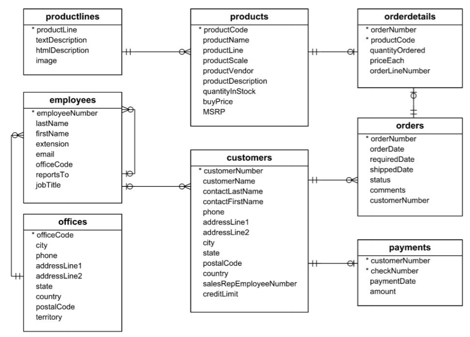
We will be using a fictional database called classicmodels from the MySQL Tutorial website. I will also use a number of examples provided in their tutorials, which is useful for comparing and validating our results.
The sample database is for a fictional company that sells model planes, cars and so on. It comprises the follow tables:
- customers: customer details including name and address
- products: a list of models, their description, vendor, quantity in stock and prices
- productlines: includes the product line (e.g. ‘motorcycles’) and a description
- orders: sales orders placed by customers, including the date and current status
- orderdetails: details of each order, including products, quantities and prices
- payments: payments made by each customer, including the date and the amount
- employees: employees’ names, titles, offices, contact details, and supervisor
- offices: address and contact details of each office
This is shown in the following schema:
Setting up
Running the queries in SQL
There are least two ways you can perform SQL queries on this sample database:
Type queries straight into the browser using the TryIt tool provided at mysqltutorial.org; or
Load the sample database into MySQL or another database management system. Instructions on how to install MySQL can be found here. Instructions on how to load in the sample database can be found here (just substitute the SQL file referred to the video with the one being used in this exercise). The SQL file for the ‘classicmodel’ database can be downloaded from mysqltutorial.org.
Running the code in R
We will be looking at equivalent R code using the dplyr package. This includes the use of the pipe operator, %>%, which allows you to chain code together in a series of logical steps. We can load the dplyr package as part of the tidyverse package:
library(tidyverse)When running the code in R, we will create a data frame that corresponds to each table in the relational database. These tables can be downloaded as individual .csv files here. Load the data into R using the following code:
# Enter the file path to where the files are saved on your system
filepath <- 'tables/'

# Read in the tables
customers    <- read_csv(paste0(filepath,'customers.csv'), na = "NULL")
employees    <- read_csv(paste0(filepath,'employees.csv'), na = "NULL")
offices      <- read_csv(paste0(filepath,'offices.csv'), na = "NULL")
orderdetails <- read_csv(paste0(filepath,'orderdetails.csv'), na = "NULL")
orders       <- read_csv(paste0(filepath,'orders.csv'), na = "NULL")
payments     <- read_csv(paste0(filepath,'payments.csv'), na = "NULL")
productlines <- read_csv(paste0(filepath,'productlines.csv'), na = "NULL")
products     <- read_csv(paste0(filepath,'products.csv'),
               # prevent the model scale (e.g. 1:10) from being read as a date:
               col_types = cols (productScale = col_character()), na = "NULL")
Now we’re ready to start running SQL queries and the equivalent code in R!
(Top)
1. Selecting data
1.1 Select all columns
The most simple select statement is one that returns all the information from a table.
With SQL:
To get data from a table in SQL we use the SELECT statement, to list the columns we are interested in, and FROM, to specify the table. If we want all records from a table, we use SELECT *. For example, to see all the records on the employees table we would use:
SELECT *
FROM employees
With R:
To get the same results in R, we simply enter the name of table, as follows:
employeesThis gives us the names and details of the 23 employees in the database:
| employeeNumber | lastName | firstName | extension | officeCode | reportsTo | jobTitle | |
|---|---|---|---|---|---|---|---|
| 1002 | Murphy | Diane | x5800 | dmurphy@classicmodelcars.com | 1 | NA | President |
| 1056 | Patterson | Mary | x4611 | mpatterso@classicmodelcars.com | 1 | 1002 | VP Sales |
| 1076 | Firrelli | Jeff | x9273 | jfirrelli@classicmodelcars.com | 1 | 1002 | VP Marketing |
| 1088 | Patterson | William | x4871 | wpatterson@classicmodelcars.com | 6 | 1056 | Sales Manager (APAC) |
| 1102 | Bondur | Gerard | x5408 | gbondur@classicmodelcars.com | 4 | 1056 | Sale Manager (EMEA) |
| 1143 | Bow | Anthony | x5428 | abow@classicmodelcars.com | 1 | 1056 | Sales Manager (NA) |
| 1165 | Jennings | Leslie | x3291 | ljennings@classicmodelcars.com | 1 | 1143 | Sales Rep |
| 1166 | Thompson | Leslie | x4065 | lthompson@classicmodelcars.com | 1 | 1143 | Sales Rep |
| 1188 | Firrelli | Julie | x2173 | jfirrelli@classicmodelcars.com | 2 | 1143 | Sales Rep |
| 1216 | Patterson | Steve | x4334 | spatterson@classicmodelcars.com | 2 | 1143 | Sales Rep |
| 1286 | Tseng | Foon Yue | x2248 | ftseng@classicmodelcars.com | 3 | 1143 | Sales Rep |
| 1323 | Vanauf | George | x4102 | gvanauf@classicmodelcars.com | 3 | 1143 | Sales Rep |
| 1337 | Bondur | Loui | x6493 | lbondur@classicmodelcars.com | 4 | 1102 | Sales Rep |
| 1370 | Hernandez | Gerard | x2028 | ghernande@classicmodelcars.com | 4 | 1102 | Sales Rep |
| 1401 | Castillo | Pamela | x2759 | pcastillo@classicmodelcars.com | 4 | 1102 | Sales Rep |
| 1501 | Bott | Larry | x2311 | lbott@classicmodelcars.com | 7 | 1102 | Sales Rep |
| 1504 | Jones | Barry | x102 | bjones@classicmodelcars.com | 7 | 1102 | Sales Rep |
| 1611 | Fixter | Andy | x101 | afixter@classicmodelcars.com | 6 | 1088 | Sales Rep |
| 1612 | Marsh | Peter | x102 | pmarsh@classicmodelcars.com | 6 | 1088 | Sales Rep |
| 1619 | King | Tom | x103 | tking@classicmodelcars.com | 6 | 1088 | Sales Rep |
| 1621 | Nishi | Mami | x101 | mnishi@classicmodelcars.com | 5 | 1056 | Sales Rep |
| 1625 | Kato | Yoshimi | x102 | ykato@classicmodelcars.com | 5 | 1621 | Sales Rep |
| 1702 | Gerard | Martin | x2312 | mgerard@classicmodelcars.com | 4 | 1102 | Sales Rep |
1.2 Select specific columns
What if you only want a subset of columns from a given table, such as employees’ first and last names?
With SQL:
In SQL you just list the column of interest in the SELECT clause as follows:
SELECT
  firstName, lastName
FROM
  employees
With R:
The equivalent R code uses the select() function:
employees %>%
  select(firstName, lastName)
Note for those learning R, it might be helpful to read the %>% operator as “and then”.
(Top)
1.3 Select distinct records
Say we want a list of distinct countries in which we have customers, i.e. without returning the same country name twice.
With SQL:
In SQL we would use SELECT DISTINCT clause, as follows:
SELECT
  DISTINCT country
FROM customers
With R:
In R, we get the same result using the distinct() function:
customers %>%
distinct(country) | country |
|---|
| France |
| USA |
| Australia |
| Norway |
| Poland |
| Germany |
| Spain |
| Sweden |
| Denmark |
| Singapore |
| Portugal |
| Japan |
| Finland |
| UK |
| Ireland |
| Canada |
| Hong Kong |
| Italy |
| Switzerland |
| Netherlands |
| Belgium |
| New Zealand |
| South Africa |
| Austria |
| Philippines |
| Russia |
| Israel |
1.4 Select distinct records with multiple columns
A similar approach can be used when you want to see distinct combinations of two or more variables / columns.
For instance, say you want a list of all US cities in which the company has customers. We can’t simply look at distinct city names, as there can be more than one city with the same name: for example, in our database we have a ‘Glendale’ in California and a ‘Glendale’ in Connecticut.
To address this we specify both city and state in our query, as follows (I’m jumping forward here and also adding a WHERE clause, to restrict our results to cities in the USA):
With SQL:
SELECT
  DISTINCT city,state
FROM
  customers
WHERE
  country = 'USA'
With R:
The equivalent R code uses filter() instead of SQL’s WHERE, as will be discussed later:
customers %>%
  filter(country == 'USA') %>%  # ignore this for now!
  distinct(city, state)
Both approaches return 24 rows containing distinct combinations of cities and states.
| city | state |
|---|---|
| Las Vegas | NV |
| San Rafael | CA |
| San Francisco | CA |
| NYC | NY |
| Allentown | PA |
| Burlingame | CA |
| New Haven | CT |
| Cambridge | MA |
| Bridgewater | CT |
| Brickhaven | MA |
| Pasadena | CA |
| Glendale | CA |
| San Diego | CA |
| White Plains | NY |
| New Bedford | MA |
| Newark | NJ |
| Philadelphia | PA |
| Los Angeles | CA |
| Boston | MA |
| Nashua | NH |
| Glendale | CT |
| San Jose | CA |
| Burbank | CA |
| Brisbane | CA |
1.5 Create new columns
What if we want to create a new column, using the information contained in existing columns?
For example: The orderdetails table contains information on which products were included in each order (productCode), the quantity of each product (quantityOrdered) and the price per unit (priceEach). We could use this information to calculate the value of each product that was ordered.
With SQL:
In SQL, within the SELECT clause, we can calculate our new column and as assign it a name (‘alias’) using the AS keyword, as follows:
SELECT
  orderNumber,
  productCode,
  quantityOrdered * priceEach AS value
FROM orderdetails
With R:
In R we would acheive the same results using the mutate function to create our new column:
orderdetails %>%
  mutate(value = quantityOrdered * priceEach) %>%
  select(orderNumber, productCode, value)
The two sets of code return 2,996 records that show the value of each product in every order. The first 20 rows are displayed in the table below:
| orderNumber | productCode | value |
|---|---|---|
| 10100 | S18_1749 | 4080.00 |
| 10100 | S18_2248 | 2754.50 |
| 10100 | S18_4409 | 1660.12 |
| 10100 | S24_3969 | 1729.21 |
| 10101 | S18_2325 | 2701.50 |
| 10101 | S18_2795 | 4343.56 |
| 10101 | S24_1937 | 1463.85 |
| 10101 | S24_2022 | 2040.10 |
| 10102 | S18_1342 | 3726.45 |
| 10102 | S18_1367 | 1768.33 |
| 10103 | S10_1949 | 5571.80 |
| 10103 | S10_4962 | 5026.14 |
| 10103 | S12_1666 | 3284.28 |
| 10103 | S18_1097 | 3307.50 |
| 10103 | S18_2432 | 1283.48 |
| 10103 | S18_2949 | 2489.13 |
| 10103 | S18_2957 | 2164.40 |
| 10103 | S18_3136 | 2173.00 |
| 10103 | S18_3320 | 3970.26 |
| 10103 | S18_4600 | 3530.52 |
2. Sorting and ordering data
2.1 Basic sorting
Data can be sorted using the ORDER BY clause in SQL and the arrange() function in R. For example, say you wanted to sort customer locations in the USA alphabetically, first by state and then by city:
With SQL:
SELECT
  DISTINCT state, city
FROM
  customers
WHERE
  country = 'USA'
ORDER BY
  state, city
With R:
customers %>%
  filter(country == 'USA') %>%
  distinct(state, city) %>%
arrange(state, city)| city | state |
|---|---|
| Brisbane | CA |
| Burbank | CA |
| Burlingame | CA |
| Glendale | CA |
| Los Angeles | CA |
| Pasadena | CA |
| San Diego | CA |
| San Francisco | CA |
| San Jose | CA |
| San Rafael | CA |
| Bridgewater | CT |
| Glendale | CT |
| New Haven | CT |
| Boston | MA |
| Brickhaven | MA |
| Cambridge | MA |
| New Bedford | MA |
| Nashua | NH |
| Newark | NJ |
| Las Vegas | NV |
| NYC | NY |
| White Plains | NY |
| Allentown | PA |
| Philadelphia | PA |
2.2 Sort descending
What if you wanted to list states in reverse alphabetical order, while listing cities in alphabetical order?
With SQL:
In SQL, you can use ORDER BY .... DESC. Any columns listed before the DESC clause will be listed in descending order.
SELECT
  DISTINCT state, city
FROM
  customers
WHERE
  country = 'USA'
ORDER BY
  state DESC, city
With R:
Equivalently, in R, you can use arrange(desc()), where the parentheses include the name of the column(s) you want listed in descending order:
customers %>%
  filter(country == 'USA') %>%
  distinct(state, city) %>%
arrange(desc(state), city) | city | state |
|---|---|
| Allentown | PA |
| Philadelphia | PA |
| NYC | NY |
| White Plains | NY |
| Las Vegas | NV |
| Newark | NJ |
| Nashua | NH |
| Boston | MA |
| Brickhaven | MA |
| Cambridge | MA |
| New Bedford | MA |
| Bridgewater | CT |
| Glendale | CT |
| New Haven | CT |
| Brisbane | CA |
| Burbank | CA |
| Burlingame | CA |
| Glendale | CA |
| Los Angeles | CA |
| Pasadena | CA |
| San Diego | CA |
| San Francisco | CA |
| San Jose | CA |
| San Rafael | CA |
2.3 Limiting the number of results
To limit the number of results that are shown, you can use SQL’s LIMIT clause and R’s slice() function. These can be combined with ordered data to return the top or bottom results from a table.
For example, if you wanted to return the five customers with the highest credit limits you could use the following:
With SQL:
SELECT
  customerName, creditLimit
FROM
  customers
ORDER BY
  creditLimit DESC
LIMIT 5
With R:
customers %>%
  select(customerName, creditLimit) %>%
  arrange(desc(creditLimit)) %>%
slice(1:5)| customerName | creditLimit |
|---|---|
| Euro+ Shopping Channel | 227600 |
| Mini Gifts Distributors Ltd. | 210500 |
| Vida Sport, Ltd | 141300 |
| Muscle Machine Inc | 138500 |
| AV Stores, Co. | 136800 |
Another option in R would be to use the top_n() function, as described here.
3. Filtering
3.1 Basic filtering
Filtering is used to restrict our results to records / rows that satisfy one or more criteria. We already saw some basic filtering in the above, in which we used SQL’s WHERE clause and R’s filter() to only shows cities that were within the United States.
Another example would be to find the names of each employee whose job title is ‘Sales Rep’:
With SQL:
SELECT
  lastName, firstName, jobTitle
FROM
  employees
WHERE
  jobTitle = 'Sales Rep'
With R:
employees %>%
  filter(jobTitle == 'Sales Rep') %>%
  select(firstName,lastName,jobTitle)
Both sets of code return the names of the 17 sales reps:
| firstName | lastName | jobTitle |
|---|---|---|
| Leslie | Jennings | Sales Rep |
| Leslie | Thompson | Sales Rep |
| Julie | Firrelli | Sales Rep |
| Steve | Patterson | Sales Rep |
| Foon Yue | Tseng | Sales Rep |
| George | Vanauf | Sales Rep |
| Loui | Bondur | Sales Rep |
| Gerard | Hernandez | Sales Rep |
| Pamela | Castillo | Sales Rep |
| Larry | Bott | Sales Rep |
| Barry | Jones | Sales Rep |
| Andy | Fixter | Sales Rep |
| Peter | Marsh | Sales Rep |
| Tom | King | Sales Rep |
| Mami | Nishi | Sales Rep |
| Yoshimi | Kato | Sales Rep |
| Martin | Gerard | Sales Rep |
There are a couple of differences to note between SQL and R:
- R uses
==instead of=when filtering - In R, it is often necessary to use
filter()beforeselect(). This would be the case if the column you are filtering on (in this case ‘jobTitle’) was not also included in theselect()function below. In SQL, this order is not an issue - In R, the filter condition is case sensitive, but in SQL it is not
(Top)
3.2 Filtering based on inequalities
We can use the ‘not equal to’ operator != to filter records that do not match a certain criteria.
For example, to see the names of the six employees who are not sales reps:
With SQL:
SELECT
  lastName, firstName, jobTitle
FROM
  employees
WHERE
  jobTitle != 'Sales Rep'
MySQL would also accept <> as the operator in this case.
With R:
employees %>%
  filter(jobTitle != 'Sales Rep') %>%
  select(lastName, firstName, jobTitle)
If you are dealing with numeric data, you can also filter using the operators >, >=, < and <=, which are the same in both languages.
(Top)
3.3 Filtering with AND conditions
Sometime we want to select rows where multiple criteria all hold true. This can be done using AND operator in SQL, and the & operator in R.
For example, if we wanted to see the names of customers who are located in California and who have a credit limit over $100,000:
With SQL:
SELECT
  customername, state, creditlimit
FROM
  customers
WHERE
  state = 'CA' AND creditlimit > 100000
With R:
customers %>%
  filter(state == 'CA' & creditLimit > 100000) %>%
  select(customerName, state, creditLimit)
These sets of code return the three customers who are both located in California and have credit limits over $100,000:
| customerName | state | creditLimit |
|---|---|---|
| Mini Gifts Distributors Ltd. | CA | 210500 |
| Collectable Mini Designs Co. | CA | 105000 |
| Corporate Gift Ideas Co. | CA | 105000 |
3.4 Filtering with OR conditions
The OR condition returns rows where any of our criteria are satisfied. In SQL we use the OR operator, while in R the | symbol is used.
For example, say we want to see a list of all customers who are located in the US or France:
With SQL:
SELECT
  customerName, country
FROM
  customers
WHERE
  country = 'USA' OR country =  'FRANCE'
With R:
customers %>%
  filter (country == 'USA' | country == 'France') %>%
  select(customerName, country)
This gives us the 48 customers who are located in either USA or France:
| customerName | country |
|---|---|
| Atelier graphique | France |
| Signal Gift Stores | USA |
| La Rochelle Gifts | France |
| Mini Gifts Distributors Ltd. | USA |
| Mini Wheels Co. | USA |
| Land of Toys Inc. | USA |
| Saveley & Henriot, Co. | France |
| Muscle Machine Inc | USA |
| Diecast Classics Inc. | USA |
| Technics Stores Inc. | USA |
| American Souvenirs Inc | USA |
| Daedalus Designs Imports | France |
| La Corne D’abondance, Co. | France |
| Cambridge Collectables Co. | USA |
| Gift Depot Inc. | USA |
| Vitachrome Inc. | USA |
| Auto-Moto Classics Inc. | USA |
| Online Mini Collectables | USA |
| Toys4GrownUps.com | USA |
| Mini Caravy | France |
| Boards & Toys Co. | USA |
| Collectable Mini Designs Co. | USA |
| Alpha Cognac | France |
| Lyon Souveniers | France |
| Auto Associés & Cie. | France |
| Marta’s Replicas Co. | USA |
| Mini Classics | USA |
| Mini Creations Ltd. | USA |
| Corporate Gift Ideas Co. | USA |
| Tekni Collectables Inc. | USA |
| Classic Gift Ideas, Inc | USA |
| Men ‘R’ US Retailers, Ltd. | USA |
| Marseille Mini Autos | France |
| Reims Collectables | France |
| Gifts4AllAges.com | USA |
| Online Diecast Creations Co. | USA |
| Collectables For Less Inc. | USA |
| Auto Canal+ Petit | France |
| Classic Legends Inc. | USA |
| Gift Ideas Corp. | USA |
| The Sharp Gifts Warehouse | USA |
| Super Scale Inc. | USA |
| Microscale Inc. | USA |
| FunGiftIdeas.com | USA |
| West Coast Collectables Co. | USA |
| Motor Mint Distributors Inc. | USA |
| Signal Collectibles Ltd. | USA |
| Diecast Collectables | USA |
3.5 Filtering with both OR, AND conditions
The examples above can be extended to combine the OR and AND conditions.
For example, if you wanted a list of customers with a credit limit of over $100,000 who are located in either the USA or France:
With SQL:
SELECT
  customerName, country, creditLimit
FROM
  customers
WHERE
  (country = 'USA' OR country =  'FRANCE') AND creditLimit > 100000
With R:
customers %>%
  filter(
    (country == 'USA' | country == 'France') & creditLimit > 100000
    ) %>%
  select(customerName, country, creditLimit)
The code above returns the 11 customers who are located in the USA or France, and who have credit limits over $100,000.
| customerName | country | creditLimit |
|---|---|---|
| La Rochelle Gifts | France | 118200 |
| Mini Gifts Distributors Ltd. | USA | 210500 |
| Land of Toys Inc. | USA | 114900 |
| Saveley & Henriot, Co. | France | 123900 |
| Muscle Machine Inc | USA | 138500 |
| Diecast Classics Inc. | USA | 100600 |
| Collectable Mini Designs Co. | USA | 105000 |
| Marta’s Replicas Co. | USA | 123700 |
| Mini Classics | USA | 102700 |
| Corporate Gift Ideas Co. | USA | 105000 |
| Online Diecast Creations Co. | USA | 114200 |
By default both SQL and R evaluate the AND operator before the OR operator. This is why it was necessary to put the OR condition in parentheses above, to tell SQL/R to evaluate it first.
If we hadn’t used parentheses, the code would have returned the list of customers who either (a) were located in the USA, or (b) were located in France and had a credit limit greater than $100,000. This would have returned the following 38 customers:
| customerName | country | creditLimit |
|---|---|---|
| Signal Gift Stores | USA | 71800 |
| La Rochelle Gifts | France | 118200 |
| Mini Gifts Distributors Ltd. | USA | 210500 |
| Mini Wheels Co. | USA | 64600 |
| Land of Toys Inc. | USA | 114900 |
| Saveley & Henriot, Co. | France | 123900 |
| Muscle Machine Inc | USA | 138500 |
| Diecast Classics Inc. | USA | 100600 |
| Technics Stores Inc. | USA | 84600 |
| American Souvenirs Inc | USA | 0 |
| Cambridge Collectables Co. | USA | 43400 |
| Gift Depot Inc. | USA | 84300 |
| Vitachrome Inc. | USA | 76400 |
| Auto-Moto Classics Inc. | USA | 23000 |
| Online Mini Collectables | USA | 68700 |
| Toys4GrownUps.com | USA | 90700 |
| Boards & Toys Co. | USA | 11000 |
| Collectable Mini Designs Co. | USA | 105000 |
| Marta’s Replicas Co. | USA | 123700 |
| Mini Classics | USA | 102700 |
| Mini Creations Ltd. | USA | 94500 |
| Corporate Gift Ideas Co. | USA | 105000 |
| Tekni Collectables Inc. | USA | 43000 |
| Classic Gift Ideas, Inc | USA | 81100 |
| Men ‘R’ US Retailers, Ltd. | USA | 57700 |
| Gifts4AllAges.com | USA | 41900 |
| Online Diecast Creations Co. | USA | 114200 |
| Collectables For Less Inc. | USA | 70700 |
| Classic Legends Inc. | USA | 67500 |
| Gift Ideas Corp. | USA | 49700 |
| The Sharp Gifts Warehouse | USA | 77600 |
| Super Scale Inc. | USA | 95400 |
| Microscale Inc. | USA | 39800 |
| FunGiftIdeas.com | USA | 85800 |
| West Coast Collectables Co. | USA | 55400 |
| Motor Mint Distributors Inc. | USA | 72600 |
| Signal Collectibles Ltd. | USA | 60300 |
| Diecast Collectables | USA | 85100 |
3.6 The IN operator
In SQL, the IN clause is used select records where a value matches any value in a list or a subquery (we’ll look at subqueries later). The equivalent operator in R is %in%.
When used on a list, the IN clause acts just like one or more OR conditions.
For example, say we want a list of customers located in either France, USA or Australia:
With SQL:
SELECT
  customerName, country
FROM
  customers
WHERE
  country IN ('France', 'USA', 'Australia')
With R:
With R, we need to combine the countries into a list using c(...):
customers %>%
  filter(country %in% c('France','USA','Australia')) %>%
select(customerName, country)| customerName | country |
|---|---|
| Atelier graphique | France |
| Signal Gift Stores | USA |
| Australian Collectors, Co. | Australia |
| La Rochelle Gifts | France |
| Mini Gifts Distributors Ltd. | USA |
| Mini Wheels Co. | USA |
| Land of Toys Inc. | USA |
| Saveley & Henriot, Co. | France |
| Muscle Machine Inc | USA |
| Diecast Classics Inc. | USA |
| Technics Stores Inc. | USA |
| American Souvenirs Inc | USA |
| Daedalus Designs Imports | France |
| La Corne D’abondance, Co. | France |
| Cambridge Collectables Co. | USA |
| Gift Depot Inc. | USA |
| Vitachrome Inc. | USA |
| Auto-Moto Classics Inc. | USA |
| Online Mini Collectables | USA |
| Toys4GrownUps.com | USA |
| Mini Caravy | France |
| Boards & Toys Co. | USA |
| Collectable Mini Designs Co. | USA |
| Alpha Cognac | France |
| Lyon Souveniers | France |
| Auto Associés & Cie. | France |
| Anna’s Decorations, Ltd | Australia |
| Souveniers And Things Co. | Australia |
| Marta’s Replicas Co. | USA |
| Mini Classics | USA |
| Mini Creations Ltd. | USA |
| Corporate Gift Ideas Co. | USA |
| Tekni Collectables Inc. | USA |
| Australian Gift Network, Co | Australia |
| Classic Gift Ideas, Inc | USA |
| Men ‘R’ US Retailers, Ltd. | USA |
| Marseille Mini Autos | France |
| Reims Collectables | France |
| Gifts4AllAges.com | USA |
| Online Diecast Creations Co. | USA |
| Collectables For Less Inc. | USA |
| Auto Canal+ Petit | France |
| Classic Legends Inc. | USA |
| Gift Ideas Corp. | USA |
| The Sharp Gifts Warehouse | USA |
| Super Scale Inc. | USA |
| Microscale Inc. | USA |
| FunGiftIdeas.com | USA |
| Australian Collectables, Ltd | Australia |
| West Coast Collectables Co. | USA |
| Motor Mint Distributors Inc. | USA |
| Signal Collectibles Ltd. | USA |
| Diecast Collectables | USA |
3.7 The NOT IN operator
If we are interested in values are not in a list - for example, all customers who are not located in France, USA or Australia?
With SQL:
In SQL we can use the NOT IN operator:
SELECT
  customerName, country
FROM
  customers
WHERE
  country NOT IN ('France','USA', 'Australia')
With R:
In R, we negate the %in% operator by placing a ! at the start of the filter function, as follows:
customers %>%
  filter(!country %in% c('France','USA','Australia')) %>%
  select(customerName, country)
Each approach gives us 69 customers who are located in countries other than France, USA or Australia.
(Top)
3.8 Filtering with regular expressions
You can filter your results based on whether a column contains characters that follow a specified pattern. For example, you may want to find names that start with the letter ‘T’, or phone numbers that include the area code ‘214’.
SQL offers a user-friendly way to do this using the LIKE operator, which is explained here. However, we are instead going to look at regular expressions, which are more flexible than SQL’s LIKE operator (though less user-friendly) and are consistent between SQL and R.
To use regular expressions in SQL we use the REGEXP operator, and in R we use the str_detect() (‘string detect’) function.
To see how this works, say we want to find all products with the word ‘Ford’ in them. We could use the following code:
With SQL:
SELECT
  productName
FROM
  products
WHERE
  productName REGEXP 'Ford'
With R:
products %>%
  filter(str_detect(productName,'Ford')) %>%
  select(productName)
These sets of code return a list of 15 models with that include the word ‘Ford’:
| productName |
|---|
| 1968 Ford Mustang |
| 1969 Ford Falcon |
| 1940 Ford Pickup Truck |
| 1911 Ford Town Car |
| 1932 Model A Ford J-Coupe |
| 1926 Ford Fire Engine |
| 1913 Ford Model T Speedster |
| 1934 Ford V8 Coupe |
| 1903 Ford Model A |
| 1976 Ford Gran Torino |
| 1940s Ford truck |
| 1957 Ford Thunderbird |
| 1912 Ford Model T Delivery Wagon |
| 1940 Ford Delivery Sedan |
| 1928 Ford Phaeton Deluxe |
The main difference in the code above is that SQL is not case sensitive but R is. You can specify case sensitivity as follows:
- To make SQL case sensitive, replace
REGEXPwithREGEXP BINARY - To make R ignore cases, replace
str_detect(productName,'Ford')in the example above withstr_detect(productName, regex('ford', ignore_case=TRUE))
The beauty of SQL’s REGEXP and R’s str_detect() is that they will both work with many of the same regular expressions. You can modify both sets of code above to see the following:
- Use the
^symbol to match the beginning of a string. For example, use'^America'to show products beginning with the words ‘America’ or ‘American’. - Use
$to denote the end of a string. For example, use'ter$'to return the names of all products that end in these three letters, such as ‘helicopter’ and ‘roadster’. - Use
'[...]'to match any of the strings listed within the brackets, which are separated with|. For example, use'^[A|B|C]'to match words beginning with either A, B, or C.
We won’t go into the details of regular expressions here, but a further explanation can be found at mysqltutorial.org.
(Top)Part 2 of this post, to follow, will look at joins, using grouped data, and subqueries.