Generating random correlated data
Summary
When carrying out financial modeling we are often interested in the range of potential outcomes. Simulations can be used to assess the distribution of possible outcomes, by treating certain inputs into our model as random. If the simulations involve more than one input, and these inputs are correlated in ‘real life’, then we need to ensure that our simulated data also reflect this correlation. This post shows how correlated random data can be produced in R and Excel for this purpose.
Intro
When producing financial models, simulations are often used to assess the range of potential outcomes. ‘Monte Carlo’ analysis involves running the model a large number of times using randomly generated data. The results of the separate trials are then combined to assess the probability of a given outcome.
If your model is based two or more variables that are correlated in real life then it is important that your simulated data be similarly correlated. This blog post aims to do the following:
- Demonstrate the importance of reflecting correlations in our simulated data;
- Identify the code that can be used to generate random correlated data, using R; and
- Briefly explains how to simulate correlated data in Microsoft Excel
Example
Assume an investor is considering buying a mixed-use property near the central business district (CBD). The property has three units. The top two floors are apartments (unit A and unit B) and the ground floor is a retail space (unit C). Each of these units currently has a rent of $2,000 per month.
The investor would like to estimate the rental income generated by the building in 5 years’ time. Among other things, this would affect the price at which they could re-sell the property. The expected rental income after five years can be expressed using a simple model:
\[ income = 2000(1 +growth_A)^5 + 2000(1 +growth_B)^5 + 2000(1 +growth_C)^5 \]
where \(growth_A\), \(growth_B\) and \(growth_c\) are the average annual growth rates for units A, B and C, respectively.
The investor assumes that the market rent for each unit would grow at 2% per year. However, this is subject to risk: the actual growth rates may be higher or lower than 2%. The investor may assume that the average growth rate will follow a normal (i.e. bell-shaped) distribution, with a standard deviation of 1%.
The investor believes that the growth rates are correlated. The change in market rents for units A and B are likely to be highly correlated, given that they are both residential units sharing the same physical location. Growth in apartment rent is also likely to be correlated with rent for the retail space, but to a lesser extent.
To assess the likely range of rental incomes in five years’ time, the investor could use simulations. Simulations involve generating thousands of random data points from an assumed distribution (in this case, a normal distribution with a mean of 2% and a standard deviation of 1%). They would then plug this data into their model and observe the range of results; in this case, the potential range of income from the building.
The range of the simulated outcomes will depend on whether or not correlations are taken into account. In this example, failing to reflect the correlations between unit types will underestimate the potential range of property income in five years’ time. This could lead the investor to underestimate the risk of purchasing the property.
Code to generate random simulated data
This section describes the code (using R) that can be used to generate our simulated growth rates. You can skip to the next section if you are more interested in the general principles than the nuts and bolts.
Our goal is to generate three growth rates that are normally distributed, each with a specified mean and standard deviation, and which are correlated with one another. To do this we will be using the mvrnorm function from the MASS package.
Start by loading our libraries:
library(tidyverse)
library(MASS)   # to produce multivariate correlated variables
The first step is to specify the mean growth rate for each unit (2%) and the standard deviation (1%). We also specify the correlations between the property units. We will assume the correlation between apartments (units A and B) is 0.9, while the correlation between each apartment and the retail unit (unit C) is 0.45.1 These are specified as follows:
## means of individual distributions
mu_A <- 0.02
mu_B <- 0.02
mu_C <- 0.02
## standard deviations
sd_A <- 0.01
sd_B <- 0.01
sd_C <- 0.01
## correlations
cor_AB <- 0.90
cor_AC <- 0.45
cor_BC <- 0.45
The next step is to generate our simulated growth rates. We will use 1,000 trials in our simulation; each trial consists of three rental growth rates corresponding to the three building units.
First we generate the data for our trials assuming the growth rates are correlated. A key piece of information here is the covariance matrix that is specified in the mvrnorm function. For this we need the variance of each unit’s growth rate, and its covariance with other units’ growth:
# Variance
# (= standard deviation squared)
var_A <- sd_A^2
var_B <- sd_B^2
var_C <- sd_C^2

# Covariance
# (= correlation between variables * product of their std devs)
cov_AB <- cor_AB * sd_A * sd_B
cov_AC <- cor_AC * sd_A * sd_C
cov_BC <- cor_BC * sd_B * sd_C

# Set seed so that our 'random' numbers are reproducible
set.seed(1)

# Generate normally distributed, correlated random variables
growth_cor <- mvrnorm(
  n     = 1000,
  mu    = c(mu_A, mu_B, mu_C),
  Sigma = matrix(c(var_A,  cov_AB, cov_AC,
                   cov_AB, var_B,  cov_BC,
                   cov_AC, cov_BC, var_C),
                 ncol = 3, byrow = TRUE),
  empirical = TRUE)

# Final dataframe
growth_cor <- growth_cor %>%
  as.data.frame()

names(growth_cor) <- c('growthA','growthB','growthC')
Second, for comparison, we will generate the same data as though the growth rates were uncorrelated or independent. This is the same as above, but we set the covariance between the variables to zero.
# Generate normally distributed, independent random variables

growth_ind <- mvrnorm(
  n     = 1000,
  mu    = c(mu_A, mu_B, mu_C),
  Sigma = matrix(c(var_A, 0,     0,
                   0,     var_B, 0,
                   0,     0,     var_C),
                 ncol = 3, byrow = TRUE),
  empirical = TRUE)

# Final dataframe
growth_ind <- growth_ind %>%
  as.data.frame()

names(growth_ind) <- c('growthA','growthB','growthC')
Examining the simulated data
We have now generated two sets of (simulated) rental growth data for the three units in the building. The first set assumes that the growth rates are correlated, while the second set assumes that they are independent.
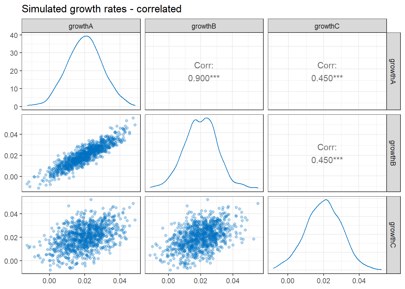
The diagram below illustrates our correlated growth rates. The 1,000 simulated growth rates are shown in the scatter plots on the bottom left. We can see that there is a high level of correlation between the growth rates for the residential units (\(growthA\) and \(growthB\)). There is also a positive correlation between these rates and rental growth for the retail unit (\(growthC\)), though the correlations are not as strong. The plots in the diagonal sections show that the distribution of the three growth rates are approximately normal.
The same charts are shown for our independent growth rates, below. Note that the variables are still normally distributed, but the scatter plots show no discernible correlation.
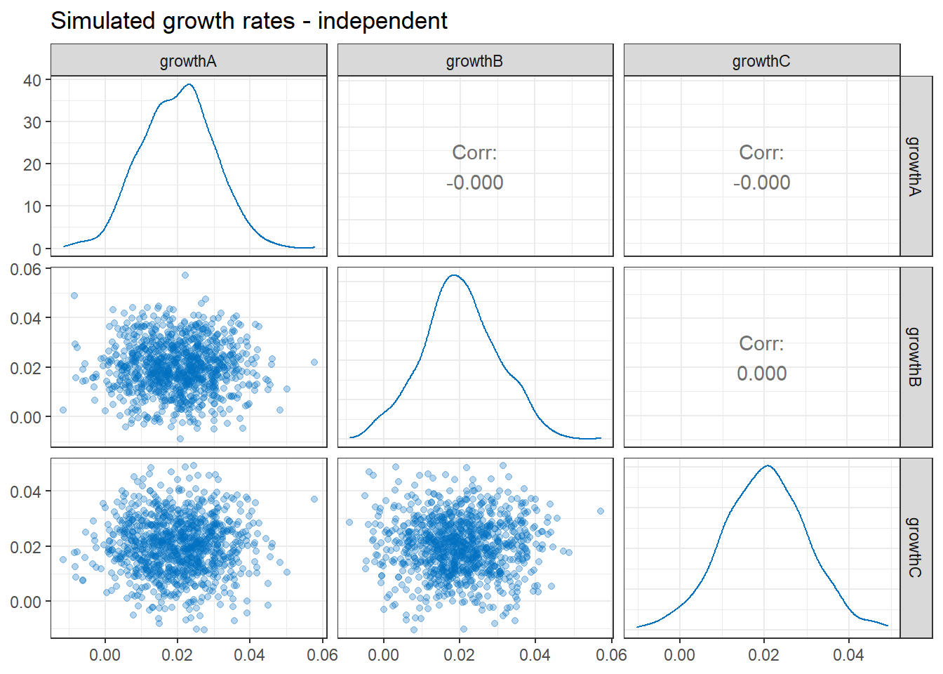
While it is not shown here, we can confirm that the mean and standard deviation of the growth rates are exactly the same in both sets of simulations above.
Implications of correlated data
We are now ready to use our simulated growth rates to assess the potential range of rental income from the property in five years’ time.
To do this, we apply the three growth rates in each trial to the formula for expected rental income:
\[ income = 2000(1 +growth_A)^5 + 2000(1 +growth_B)^5 + 2000(1 +growth_C)^5 \]
This will give us 1,000 estimates of monthly rental income five years from now.
The histogram below shows us the range of projected rental incomes (from these 1,000 trials) when both the correlated and uncorrelated growth rates are used.
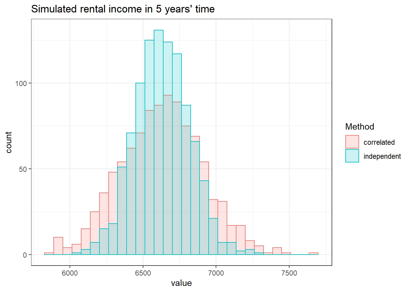
In both cases, the average monthly rental income is the same, at $6,631 per month. This is very close to what we would have got had we simply plugged the expected growth rate of 2% per year into the formula above (6,624 per month).
However the correlated growth rates give a wider range of potential rental income. The risk of the investment (as measured by the dispersion around the average value) is more apparent when our data reflects the likely correlations in rental growth rates.
Accounting for correlations can have significant implications for decision making. To illustrate, say the investor knows in advance (using discounted cash flow analysis) that the investment will only be feasible if the rent generated by the property exceeds $6,400 in five years’ time. When independent growth rates are assumed, rental income falls below this threshold in only 10.4% of trials. However, when correlations are taken into account, this doubles to 21.0% of trials.
| Method | Average | Std Dev | % of trials < $6400 |
|---|---|---|---|
| correlated | 6631 | 278 | 21.0 |
| independent | 6631 | 188 | 10.4 |
The foregoing illustrates the importance of taking correlations into account when running simulations. Failing to account for correlations could underestimate the range of potential outcomes. It could also overestimate the range of potential outcomes, depending on whether the data being simulated was positively or negatively correlated in real life, and the model used to generate the outcome of interest.2
Simulations with correlated data in Excel
In the example above we simulated multivariate data (i.e. three or more variables) with correlations using R code.
You can do something similar in Microsoft Excel. However, this depends on whether you want to simulate correlations between two variables (‘bivariate’) or three or more variables (‘multivariate’). The former is relatively straightforward, but the latter requires the use of macros or addins.
Simulating two correlated variables
The following is an example of how we can produce two random, normally-distributed variables, X and Y, with a specified correlation between the two. Note that these are random values, so your figures will be different from those shown below.
We begin by entering our parameters in the second column (see screen shot below). These include
- The mean of X (\(meanX\));
- The standard deviation of X (\(sdX\));
- The mean of Y (\(meanY\));
- The standard deviation of Y (\(sdY\)); and
- The correlation coefficient (\(rho\))
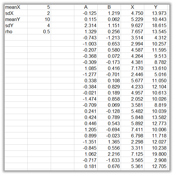
Next we create two random ‘helper’ variables, A and B, which are normally distributed with a mean of zero and a standard deviation of 1 (i.e. ‘standard normal’). To produce each of these variables we use the Excel formula =NORM.INV(RAND(),0,1). This formula can then be copied down, e.g. 1000 times, depending on how many trials you want in the simulation.
Next, create variable X. The values in this column are calculated using the general formula \(meanX+sdX \cdot A\), where A is the corresponding cell in the helper column described above.
Then create variable Y. The values in this column are are based on the formula: \(meanY + sdY (A \cdot rho+B(1-rho^2)^{0.5})\), where again A and B refer to the corresponding cells in the helper columns.
You can then check that the new variables (X and Y) have the expected means, standard deviations and correlation.
Simulating 3+ correlated variables
Simulating more than two correlated variables in Excel is more complex, and requires VBA code or an addin.
One such add in is Simtools.
I won’t go into detail on this here, but if you’re interested (or are struggling to implement it) let me know and I can provide some details.
And there you have it - I hope you found this useful.